Intro to Parameterizations in WRF
An Introduction to Parameterization Options in WRF
This post is the first in a series about parameterization schemes in WRF. We hope they will help demystify the role these schemes play in the model, so that you can make a more informed decision about which schemes to use for your own run. This post provides a very brief overview; future posts will be a more detailed look at specific scheme categories.
To understand parameterizations, we first must discuss what a model does. According to Schwarz et al. (2009), models are representations that explain and predict a natural phenomenon. In the atmospheric sciences, accuracy of the model’s prediction is directly related to how well it represents atmospheric processes, which can be adjusted by choosing the best parameterization schemes for your research question. Every choice made changes the outcome of the model simulation. As a result, parameterization schemes are one of the most important aspects to consider when setting up a computer model.
Unfortunately, choosing the best parameterization schemes is also one of the most difficult steps of the model set up procedure because there is no single “best combination”; it depends entirely on the research question you chose, the location and size of your domain, and the resolution of your domain. Even after considering these options, some choices may still not be clear.
It is not hopeless, though! It is possible to make an informed decision on which parameters to use if you understand how the different schemes influence the model.
What do parameterization schemes do?
In very general terms, here’s how parameterization schemes in WRF work:
From our current understanding of atmospheric processes, atmospheric scientists have derived several equations that describe dynamic and physical processes. In a basic sense, weather is created when there is uneven heating, creating regions of relatively warm and cool temperatures, which causes air to move (or be transported). On a spherical planet with no water or vegetation, this simple model description is probably pretty representative of how the atmosphere behaves. However, on a planet like Earth, more equations are need in order to take into account things like oceans, mountains, ice, plants and animals.
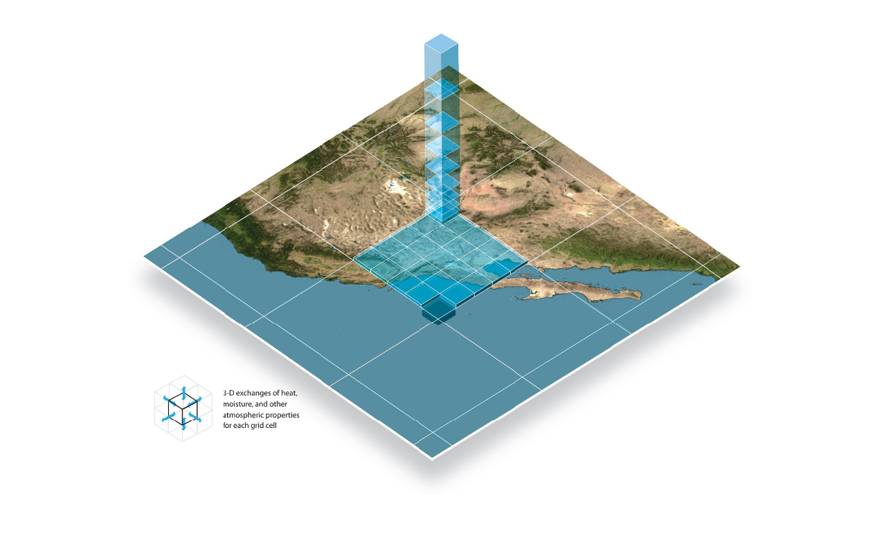
In fact, there are so many different influences and interactions to consider, that many equations are needed. Therefore, parameterization options are generally broken down into categories. In general, parameterizations use mathematical formula (derived from theoretical understanding of atmospheric processes) to calculate values for variables of interest. Stensrud (2007) summarizes most schemes into the categories of: land surface, atmosphere interaction, water-atmosphere interaction, planetary boundary layer and turbulence, convection, microphysics, and radiation. WRF uses similar distinctions, but organizes its parameterization schemes using the following structure:
-
Physics Options
-
Microphysics (mp_physics)
-
Longwave Radiation (ra_lw_physics)
-
Shortwave Radiation (ra_sw_physics)
-
Cloud fraction option
-
Surface Layer (sf_sfclay_physics)
-
Land Surface (sf_surface_physics)
-
Urban Surface (sf_urban_physics)
-
Lake Physics (sf_lake_physics)
-
Planetary Boundary Layer (bl_pbl_physics)
-
Cumulus Parameterization (cu_physics)
-
-
Diffusion and Damping Options
-
Advection Options
-
Lateral Boundary Conditions
As you can see, there are many categories with at least 2-3 scheme options per category. The result is literally hundreds of thousands of potential combinations to choose from.
Advantages and disadvantages of parameterization schemes
The equations that make up parameterization schemes in WRF range from very simple to very complex. In general, the more complex options are much more comprehensive and provide more precise and accurate results. Which begs the question: why not use the most complex, in-depth parameterizations every time, if they yield more precise results? There are several reasons, but the best explanation is: computation time is expensive.
In order to get an accurate representation of the region you are modeling, you want to create a domain that is as large as possible with the highest resolution possible. This means, as many grid points as possible. The problem is that the model solves all the equations at every grid point for every time step, therefore if the model runs for a long time period, for a large domain, or for a high resolution, the computer is doing A LOT of calculations. This can take a very long time to do, or requires lots of processors (which are expensive). Therefore, sacrifices have to be made based on the question being researched.
Climate, weather, and regional climate models
Consider, for example, a climate model versus a weather model. Weather models tend to have complex parameterizations that focus on small-scale processes, therefore also have high resolutions. The goal of weather models is to precisely and accurately forecast day to day weather. Since the resolution is high and parameterizations are complex, the models are run over a very small domain in order to be sure the model run-time is reasonably short. After all, what good is a 24 hour forecast if the model takes 48 hours to run?
Climate models, however, have a different goal. The goal is to accurately indicate trends (rather than specific values) over a very long period of time and a very large domain (often the entire planet). Therefore, parameterization schemes focus on large-scale processes and resolution is generally quite low. In the case of climate models, it is OK if the model takes several days to complete a run, since the model is usually looking at several decades into the future.
Regional climate modeling (as is frequently done using WRF) requires some combination of both processes and is why nesting is such an important part of setting up the model domain. The larger, coarser nest calculates the climate influence on the region (using large-scale, less complex processes) and the smaller, high resolution nest calculates the weather as influenced by the climate for that region (using small-scale, more complex processes). Therefore, parameterization schemes must be chosen with both of these ideas in mind.
Figure 2. Visual representation of Earth’s Climate System. Image from UCAR Digital Library.
Choosing parameterizations based on research questions
Next, consider the following hypothetical research question: Does urban development impact the wind over a wind turbine farm in my domain? In order to choose the best parameterizations for the model run, you have to think about the question being asked. First, the dynamic processes that calculate small-scale wind and speed relating to radiative heating are important and complex, in-depth parameters should be chosen. Similarly, small-scale dynamical processes and accurate representation of orography and urban structures require small grid spaces, so a high resolution is also required. However, small-scale microphysical processes that determine different concentrations of various water particles in the atmosphere is not an important component of this question. So, using a less-complex microphysics scheme will save computing power and likely will not impact the answer to your research question.
Final Thoughts
While choosing the most complex and comprehensive parameterization option may seem like the best choice, it is important to consider the resolution and size of your domain as well as the time period of your model run. When you consider your research question, be sure to ask yourself:
-
What length of time am I interested in studying: long range or short range time scales?
-
What variables am I interested in looking at: are they small-scale or large-scale?
-
Based on my variables of interest and the size of my region, do I need to use a fine resolution or is a coarse resolution ok? Is nesting an appropriate option?
-
Are my variables of interest the result of primarily dynamic processes or microphysical processes?
-
Which parameterization category options are most important? Which are least important?
This is by no means a comprehensive list of questions to consider, but it is a nice place to start. In future posts, we will take a much closer look at several microphysics, cumulus, radiation, and boundary layer options in WRF. At the end of this post series, we hope you will have a much better idea of how these schemes will impact your WRF run.
Until next time,
-Morgan
References
Schwarz, C. V., Reiser, B. J., Davis, E. A., Kenyon, L., Acher, A., Fortus, D., et al. (2009). Developing a learning progression for scientific modeling: Making scientific modeling accessible and meaningful for learners. Journal of Research in Science Teaching , 632-654.
Skamarock WC, Klemp JB, Dudhia J, et al. A description of the advanced research WRF version 2. NCAR/TN-468+STR 2005.
Stensrud D. J. (2007). Parameterization Schemes: Keys to Understanding Numerical Weather Prediction Models. Cambridge University Press, New York.