This blog features content related to science education, teaching strategies, interesting news about atmospheric science, and tools for scientific data collection and analysis. The ultimate goal of this blog is to give our volunteer contributors the opportunity to share interesting scientific information as well as practice communication strategies. Please note that constructive comments and discussion are welcome, but highly negative comments will be removed.


Contributors   


Morgan B. Yarker, PhD, CCM


Michel d. S. Mesquita, PhD


Interested in being a guest contributor? Please fill out this form and we will contact you!


AMS 2019 Activities

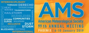
Interact with Yarker Consulting at

The AMS Annual Meeting

Yarker Consulting and its partners are heading to Phoenix this weekend for the American Meteorological Society’s (AMS’s) annual meeting. The government shutdown has had a significant impact on the conference, in largely negative ways. However, we have been working hard all year to prepare for this event and are excited to share our work, learn new things, and network with our colleagues who are able to attend. If you will be joining us in Phoenix this week, be sure to check out as many of these amazing activities as possible.

Saturday

Our intern, Antoinette Serrato, will be attending the Student Conference. Sessions include conversations with professionals, Introductions to various careers in the field, and the always popular Career Fair.

Sunday

9:00am – 3:30pm Early Career Professional Conference

One of the best things about the ECPC is the networking. This group does networking right because they provide excellent guidance and ample opportunity. In particular, the 9:00am session will include an exciting guest from Improv Science that you won’t want to miss!

Be sure to grab your lunch (included in the ECPC registration fee) and do some active learning in our Mock Trial! You will have the opportunity to evaluate scenarios from legal cases with the support of experienced Certified Consulting Meteorologists (CCMs), including our Founder, Morgan and our partner, Jared.  This event is sponsored by the Association for Consulting Meteorologists.

Other sessions include discussions about managing mental health, non-traditional careers, and outside of the box skillsets.

5:00pm – 6:15pm Early Career Professional Conference Attendee Networking Dinner

Need plans for dinner? No problem! Join the rest of the ECPC attendees for dinner and conversation. It’s a great time to get to know your peers better and meet new people!

8:00pm – 9:00pm Association for Consulting Meteorologists Informal Gathering

Have you ever thought about getting your CCM? Ever wonder what kinds of consulting work meteorologists do? This is the perfect opportunity to explore the world of consulting meteorology! Bring a friend to this informal get-together to meet current ACM members and ask those burning questions. Message our Founder (also an ACM Board Member) for more information and the location.

9:00pm -11:00pm Early Career Professionals Reception

As I said, this group does networking well! Another opportunity to mingle with other ECPs. This event is open to all, so bring a friend!

Monday

Keep an eye out for Badges that have a special sticker. AMS is piloting a brand-new Teacher Travel Grant program and is bringing six K-12 teachers from across the country to the meeting so that they can network with scientists, learn about the latest research, and collaborate with other educators. Most of these teachers have never been to AMS before, so if you see one, be sure to say “hi!”

10:30am – 12:00pm Early Career Leadership Academy

Both our Founder and Partner participated in the inaugural Early Career Leadership Academy in 2018. Learn from a few member’s experiences and future classes of ECLA. I highly recommend this program, and anyone interested should definitely attend this session!

10:30am – 12:00pm Active Learning Demonstrations

The Education Symposium is exploring alternative presentation styles with an Active Learning session Monday morning. Pop in and participate in a few demonstrations!

4:00pm – 6:00pm Education Symposium Poster Session: A Case for Entrepreneurial Meteorology

Yarker Consulting’s very own Intern, Antoinette Serrato, will be giving her first AMS presentation at this poster session! A collaborative project between Yarker Consulting, m2lab.org, and Sales and Marketing, Inc. provides a case for why students and professionals should have exposure to entrepreneurial meteorology. Be sure to stop by and say, “hi!” We would love to see you there!

Tuesday

3:00pm – 4:00pm Education Symposium: Using Alternative Presentation Formats to Inform Your Audience

As educators, we recognize the value of exploring alternative ways to present information to audiences. Our Founder is stepping in as a substitute chair for this session, where several authors will present new and innovative ways to educate.


See you in Phoenix!

-Morgan

Environment and children


3 Ways in which Climate Uncertainty is Impacting Children

Michel d. S. Mesquita, PhD


I have been part of a number of climate studies, meetings and conferences. While discussions often have focused on modeling (my field), policy, water cycle, energy, among others- very little has been about the effect climate change could have on children. But with the recent release of the Fourth National Climate Assessment, it is appropriate to consider the impact climate uncertainty has on our most vulnerable members of society.

Source: Photo by Caleb Woods on Unsplash


1. Children are one of the most vulnerable groups exposed to new disease

The Zika virus epidemic in Brazil is a recent example on how vector borne diseases have affected children already now. It’s reported that about 4,000 babies were born with microcephaly due to the Zika virus (1).  This is a condition in which a baby head is small compared to their body size, with consequences to their proper neurodevelopment.

Source: Photo by Hermes Rivera on Unsplash

The Zika virus is transmitted through the Aedes mosquito. These mosquitoes thrive in warm temperatures and water puddles left unchecked. Open sewage, as a result of improper infrastructure, is also a field for the proliferation of even more mosquitoes. Since its discovery, Zika-carrying mosquitos have migrated as far north as the Southern US, impacting communities across South, Central, and North America. In an uncertain future climate, Zika could become a major epidemic, affecting even more children.


2. Children’s life-long health is a direct result of the quality of their air

Air pollution is another threat to children’s well being. A quick Wikipedia search under the topic “street children” shows that about 100 million children grow up in the streets. Many live in large urban areas of densely populated and air polluted cities.

Source: Photo by Viktor Juric on Unsplash

When these children are exposed to smog, PM2.5 particles, which stands for particulate matter of the size of 2.5 micrometers, deposits in their lungs. They may impair the lung function, since they can penetrate deeply into the alveolar wall and bloodstream. Life-long health issues develop as a result of excessive PM2.5 exposure. For street children, health care is not an option, which is why their survival rate is not high (2). Since meteorological conditions may affect the concentration of PM2.5 in the atmosphere, a combination of future changes in weather conditions and policies concerning pollution may influence considerably the future of street children. As a result, air quality poses a threat to children’s survival.


3. Children face high levels of stress at young ages

 As environmental threats become more common and their impacts less certain, stress becomes an ever-persistent emotion, for adults as well as children. The recent California fires and the devastation of Paradise, a town located about 3 hours from San Francisco, showcases how stressful it can be for families. Many have lost their homes, others have lost their loved ones, or both. For children having to evacuate or miss their home, pets, family members, it must be devastating. Such stressful conditions could potentially affect their future development. This is just one example of an serious of natural disasters in recent years, which has put families in difficult positions physically and financially

Uncertainty in climatic conditions is already affecting children. More studies are needed to understand what the future could bring to these small ones. By then, many will have become adults and will already be seeing their own children being affected as well.


1 The Guardian (2018), URL: https://www.theguardian.com/world/2018/jul/20/zika-epidemic-sheds-light-on-brazils-invisible-children  

2 *What About America’s Homeless Children?: Hide and Seek: https://tinyurl.com/ybfxezfz

*not many studies are available on mortality, a study mentions that it can be 10 times higher compared to a regular person at the same age group.

Advanced Resources for R

An Introduction to R: Advanced Resources

These are links to various resources that help you go beyond the introductory course at m2lab.org. We hope you find them helpful!

Tutorial on how to use Google Maps to create publication-ready maps in R

R package that will allow you to work with World Bank climate data

With this package you can obtain WRF forecasts in R

A list of spatial statistics packages

Powerpoint slides from a Harvard University workshop on applied spatial statistics in R

Several instructional videos currently available on YouTube

Intro to Parameterizations in WRF

An Introduction to Parameterization Options in WRF

This post is the first in a series about parameterization schemes in WRF. We hope they will help demystify the role these schemes play in the model, so that you can make a more informed decision about which schemes to use for your own run. This post provides a very brief overview; future posts will be a more detailed look at specific scheme categories.

To understand parameterizations, we first must discuss what a model does. According to Schwarz et al. (2009), models are representations that explain and predict a natural phenomenon. In the atmospheric sciences, accuracy of the model’s prediction is directly related to how well it represents atmospheric processes, which can be adjusted by choosing the best parameterization schemes for your research question. Every choice made changes the outcome of the model simulation. As a result, parameterization schemes are one of the most important aspects to consider when setting up a computer model.

Unfortunately, choosing the best parameterization schemes is also one of the most difficult steps of the model set up procedure because there is no single “best combination”; it depends entirely on the research question you chose, the location and size of your domain, and the resolution of your domain. Even after considering these options, some choices may still not be clear.

It is not hopeless, though! It is possible to make an informed decision on which parameters to use if you understand how the different schemes influence the model.

What do parameterization schemes do?

In very general terms, here’s how parameterization schemes in WRF work:

From our current understanding of atmospheric processes, atmospheric scientists have derived several equations that describe dynamic and physical processes. In a basic sense, weather is created when there is uneven heating, creating regions of relatively warm and cool temperatures, which causes air to move (or be transported). On a spherical planet with no water or vegetation, this simple model description is probably pretty representative of how the atmosphere behaves. However, on a planet like Earth, more equations are need in order to take into account things like oceans, mountains, ice, plants and animals.

In fact, there are so many different influences and interactions to consider, that many equations are needed. Therefore, parameterization options are generally broken down into categories. In general, parameterizations use mathematical formula (derived from theoretical understanding of atmospheric processes) to calculate values for variables of interest. Stensrud (2007) summarizes most schemes into the categories of: land surface, atmosphere interaction, water-atmosphere interaction, planetary boundary layer and turbulence, convection, microphysics, and radiation. WRF uses similar distinctions, but organizes its parameterization schemes using the following structure:

  1. Physics Options

    1. Microphysics (mp_physics)

    2. Longwave Radiation (ra_lw_physics)

    3. Shortwave Radiation (ra_sw_physics)

    4. Cloud fraction option

    5. Surface Layer (sf_sfclay_physics)

    6. Land Surface (sf_surface_physics)

    7. Urban Surface (sf_urban_physics)

    8. Lake Physics (sf_lake_physics)

    9. Planetary Boundary Layer (bl_pbl_physics)

    10. Cumulus Parameterization (cu_physics)

  2. Diffusion and Damping Options

  3. Advection Options

  4. Lateral Boundary Conditions

As you can see, there are many categories with at least 2-3 scheme options per category. The result is literally hundreds of thousands of potential combinations to choose from.

Advantages and disadvantages of parameterization schemes

The equations that make up parameterization schemes in WRF range from very simple to very complex. In general, the more complex options are much more comprehensive and provide more precise and accurate results. Which begs the question: why not use the most complex, in-depth parameterizations every time, if they yield more precise results? There are several reasons, but the best explanation is: computation time is expensive.

In order to get an accurate representation of the region you are modeling, you want to create a domain that is as large as possible with the highest resolution possible. This means, as many grid points as possible. The problem is that the model solves all the equations at every grid point for every time step, therefore if the model runs for a long time period, for a large domain, or for a high resolution, the computer is doing A LOT of calculations. This can take a very long time to do, or requires lots of processors (which are expensive). Therefore, sacrifices have to be made based on the question being researched.

Figure 1. Visual representation of grid spaces in atmospheric models. Image from UCAR Digital Library.

Climate, weather, and regional climate models

Consider, for example, a climate model versus a weather model. Weather models tend to have complex parameterizations that focus on small-scale processes, therefore also have high resolutions. The goal of weather models is to precisely and accurately forecast day to day weather. Since the resolution is high and parameterizations are complex, the models are run over a very small domain in order to be sure the model run-time is reasonably short. After all, what good is a 24 hour forecast if the model takes 48 hours to run?

Climate models, however, have a different goal. The goal is to accurately indicate trends (rather than specific values) over a very long period of time and a very large domain (often the entire planet). Therefore, parameterization schemes focus on large-scale processes and resolution is generally quite low. In the case of climate models, it is OK if the model takes several days to complete a run, since the model is usually looking at several decades into the future.

Regional climate modeling (as is frequently done using WRF) requires some combination of both processes and is why nesting is such an important part of setting up the model domain. The larger, coarser nest calculates the climate influence on the region (using large-scale, less complex processes) and the smaller, high resolution nest calculates the weather as influenced by the climate for that region (using small-scale, more complex processes). Therefore, parameterization schemes must be chosen with both of these ideas in mind.

Figure 2. Visual representation of Earth’s Climate System. Image from UCAR Digital Library.

Choosing parameterizations based on research questions

Next, consider the following hypothetical research question: Does urban development impact the wind over a wind turbine farm in my domain? In order to choose the best parameterizations for the model run, you have to think about the question being asked. First, the dynamic processes that calculate small-scale wind and speed relating to radiative heating are important and complex, in-depth parameters should be chosen. Similarly, small-scale dynamical processes and accurate representation of orography and urban structures require small grid spaces, so a high resolution is also required. However, small-scale microphysical processes that determine different concentrations of various water particles in the atmosphere is not an important component of this question. So, using a less-complex microphysics scheme will save computing power and likely will not impact the answer to your research question.

Final Thoughts

While choosing the most complex and comprehensive parameterization option may seem like the best choice, it is important to consider the resolution and size of your domain as well as the time period of your model run. When you consider your research question, be sure to ask yourself:

  • What length of time am I interested in studying: long range or short range time scales?

  • What variables am I interested in looking at: are they small-scale or large-scale?

  • Based on my variables of interest and the size of my region, do I need to use a fine resolution or is a coarse resolution ok? Is nesting an appropriate option?

  • Are my variables of interest the result of primarily dynamic processes or microphysical processes?

  • Which parameterization category options are most important? Which are least important?

This is by no means a comprehensive list of questions to consider, but it is a nice place to start. In future posts, we will take a much closer look at several microphysics, cumulus, radiation, and boundary layer options in WRF. At the end of this post series, we hope you will have a much better idea of how these schemes will impact your WRF run.

Until next time,

-Morgan

References

Schwarz, C. V., Reiser, B. J., Davis, E. A., Kenyon, L., Acher, A., Fortus, D., et al. (2009). Developing a learning progression for scientific modeling: Making scientific modeling accessible and meaningful for learners. Journal of Research in Science Teaching , 632-654.

Skamarock WC, Klemp JB, Dudhia J, et al. A description of the advanced research WRF version 2. NCAR/TN-468+STR 2005.

Stensrud D. J. (2007). Parameterization Schemes: Keys to Understanding Numerical Weather Prediction Models. Cambridge University Press, New York.

The End of p Values?

The end of p values?

This is the second of a two-part post discussing the scientific journal Basic and Applied Social Psychology editor’s controversial decision to ban the use of p-values in their publications. Part one can be found here.


The Royal Statistical Society (RSS) 2015 Conference featured a debate on the use of p values. The discussant was Dr. David Colquhoun, University College London,. But why was there such a debate at the RSS conference? Earlier this year, the Basic and Applied Social Psychology (BASP) journal decided to ban the use of p values. The reason? Well, one of the reasons was that statistics might be used to support ‘lower-quality research’ (Woolston, 2015). So, the RSS debate was there to promote a discussion around the strict BASP decision and to rethink the use of p values.


The RSS 2015 debate was arguably one of the most effective scientific discussions of the year. This is because it showcased both sides of the debate (for and against) in light of sound reasoning. Also, it featured a room packed with some of the best statisticians in the world. An important outcome of the debate was that it highlighted the need for university degrees to teach their students to be more critical to what they learn. This idea makes sense, because the goal of science is to insure all claims are thoroughly critiqued; therefore it is important that all evidence is considered. p values are just one piece of evidence in any story, hence should not be the be-all and end-all for the results of the study. For example, were you taught at your university to consider the possibility that the use of p values might be flawed for the study? Have you learned other alternatives to hypothesis testing? This is an important, more constructive approach to teaching statistics in the science classroom.


What is a p value?

In hypothesis testing, p values represents the probability (or likelihood) that the result obtained is ‘more extreme’ than what would normally be observed, given a specific hypothesis. Also, one uses a threshold (significance level) above which it one would not reject the null hypothesis, and below which one would reject the null hypothesis in favor of the alternative one. A threshold of 5% is often used. The use of p values started in the 1770s and their use in statistics were later popularized by Ronald Fisher (Ibid.).


The use of p values is best done with an already existing set of large data because generally the goal is to determine if one specific set of data is unusually different from what normally happens. This can be done for either inductive or deductive processes.


Inductive and deductive

In all forms of scientific inquiry, there are two ways to draw reasonable conclusions about a topic; that is through a process of either induction or deduction. One of the first and most commonly cited definitions of inductive and deductive reasoning was written by John Dewey in 1910, who states that “…building up the idea is known as inductive discovery; the movement toward developing, applying, and testing, as deductive proof.” (p 244).


In other words, induction is about taking evidence already known and attempting to make sense of it. The example Dewey gives is to think of someone who left a room for a period of time and comes back to find objects in the room scattered about in disarray. Inductive logic would be to consider the presence of a burglar. No burglar was observed directly, but with the brief evidence provided, it seems to be the best conclusion. Using meteorology as an example, perhaps you use p values to determine that one particular rain event was statistically more intense than is usual for the area. You may suspect that something influenced this high rain event, but your p value does not tell you what that could be. At this point, you are using your information to establish evidence that something happened, but more research needs to be done to figure out what.


Deduction involves testing already existing theories. Therefore, in Dewey’s example, deduction begins once data collection and evidence derivation beings. The person may search their valuables, check windows and doors for entry marks, or perhaps anything unusual in the room that the burglar may have left behind. The idea during deductive logic is to confirm the original theory that a burglar was in the room and (potentially) identify who the burglar was. This is equivalent to using several p values to narrow down the reason for your high rain event in the meteorology example. Perhaps you use p values to explore other atmospheric phenomenon leading up to your intense precipitation event. Maybe wind direction, wind speed, and temperature values were within expected ranges, but dewpoint values were higher than normal. What caused the higher dewpoint values? Further research would have to be done. This process of continually testing and hypothesizing using p values is building evidence and is inductive reasoning.


Therefore, the problem with relying too heavily on p values is that when it is used inductively (as one piece of evidence to suggest that something is different) without following it up with further research to determine why the precipitation event is more intense than usual, we can end up with conclusions drawn from poor use of scientific inquiry, which is not how p values were intended to be used. When conclusions are drawn prematurely using p values, it is inevitable that ‘false discoveries’ occur, which can lead to a whole host of new problems.


False discovery rate

One of the major issues in the use of p values was pointed out by Colquhoun in his address at the RSS 2015. The use of a threshold of 5% leads to a number of false positive tests (or false discoveries) – leading to a false discovery rate that could be as high as 30% or more (Colquhoun, 2014). So, what threshold should one use? In Colquhoun’s talk, he emphasized that a threshold of 4% (p=0.04) does not mean one has discovered something, it only means that ‘it might be worth another look’ (Colquhoun, 2015). In order to say one has discovered something, a threshold of 0.5% or 0.1% (p value of 0.005 or 0.001, respectively) should be used (Johnson, 2013). A p value of 0.001 (or less) will give a false discovery rate of less than 2% (Colquhoun, 2015).


Concluding remarks

The p value discussion is still ongoing, but one thing is certain: we should not take what we learn at university as something for granted. One has to critically evaluate what is learned and keep apace with new ways of thinking. Most importantly, p values should be used in deductive reasoning; as a way to derive a variety of evidence to support a conclusion. Not as a be-all and end-all to draw conclusions. Finally, when working with hypothesis testing, one needs to think about the following points:

  • If you still decide to use p values, use them with caution. Be sure it is one piece of a variety of evidence, not the only piece of evidence.
  • Remind yourself that a 5% threshold has a high false discovery rate, so you would be “wrong at least 30% of the time” (Colquhoun, 2014)
  • Conduct tests at the 0.005 or 0.001 level of significance (Johnson, 2013) and according to Colquhoun (2014): “never use the word ‘significant’”. It is easily confused with meaningful.


– Michel and Morgan


References:
Colquhoun, D. (2015). “P-values debate.” Retrieved 28 October, 2015, from https://rss.conference-services.net/programme.asp?conferenceID=4494&action=prog_list&session=33652
Colquhoun, D. (2014). "An investigation of the false discovery rate and the misinterpretation of p-values." Royal Society Open Science 1(3).
Dewey (1910): Systematic Inference: Induction and Deduction. How We Think. D.C. Heath & Company.
Johnson, V. E. (2013). "Revised standards for statistical evidence." Proceedings of the National Academy of Sciences 110(48): 19313-19317.
Woolston, C. (2015). Pscychology journal bans P values. Nature, Macmillan Publishers Limited. 519: 9.


Data Assimilation Overview

Data Assimilation in WRF: An Overview

One of the greatest benefits to using atmospheric computer models is the ability to experimentally test the influence of new and unusual forces on weather and climate. Have you ever wanted to include additional data into your WRF run? Perhaps you have sea surface temperature, a specific set of precipitation, or other kinds of data. Maybe your research question requires a special set of data in your simulation. This post provides an overview of data assimilation techniques to help you get started on this process.


Sea-Surface Temperature

Although WRF doesn’t require sea-surface temperature (SST) to run, if you are doing longer simulations (like those you would do for regional climate modeling), it can be very beneficial. Therefore, WRF was designed to seamlessly incorporate SST into simulations. They even created a tutorial online with a link to free data to help you get started. This is probably the easiest way to get started with data assimilation, if you are new to WRF.


WRFDA

Did you know that WRF has a data assimilation component available? It’s called WRFDA and is described in chapter 6 of the WRF User’s Guide. It provides step-by-step descriptions of how to assimilate a few commonly used types of data, such as radiance, radar, and precipitation. It even provides some free input data you can use in your run, so this is an excellent place to start.


Be aware that if you have already installed the full version of WRF, you will still need to download and install the WRFDA component. Don’t worry though, if you managed to get WRF installed, the assimilation component should be pretty straightforward and integrate seamlessly.


Modifying the Source Code

This process is the most difficult to do, but it gives you the most flexibility. For example, let’s say you want to see if the heat released from a volcano eruption impacted the weather in your domain. You would want to replace land-surface temperature for that one specific grid cell, which would have to be done by finding the variable in the source code and modifying it. If you are interested, this is exactly what I did for my Masters Thesis, which has been published and is free to access.


Heat from a volcano comes from the use of satellite data. Once you have obtained a reasonable dataset, you will have to be sure you have interpolated the data to match the timestep (“time_step” in your namelist file) for the number of days, hours, minutes, etc. You have to be sure the amount of data you have matches the number of iterations WRF will use.


You also need to decide how to introduce the data into WRF for the run. This requires thoughtful consideration of the components of WRF as well as the parameterization schemes you decided to use (which you specified in your namelist). Eventually, you will have to explore the WRF source code for the equations and variables you are interested in. However, you risk making accidental changes if you are continually opening and closing files, which may alter how the model works or even prevent it from running altogether. So I suggest using an online source file, such as this one, so you can search the files without fear of risking your WRF code. Additionally, the files are all easily sorted so you don’t have to change directories as you are searching either. Once you know exactly what you want to modify, you can edit the correct file in code on your computer.


Screenshot of the WRF code browser


To incorporate heat from the volcano, you are changing the long-wave radiation output from the one grid cell that the volcano is in. Assume you are using the RRTM, you would search through that source code for the variable describing surface temperature. At the beginning of the RRTM subroutine, they list the variables:

SUBROUTINE RRTM (TTEN,GLW,OLR,TSFC,CLDFRA,T,Tw,QV,QC,              & 1,5
                  QR,QI,QS,QG,P,Pw,DZ,                              &

                  EMISS,R,G,                                        &
                  kts,kte                                           )

As you would expect, temperature is identified with a “T”, therefore, we will look to see when T is first used in calculations later on in the code. If you scroll down, you should come across the following: 

CALL MM5ATM (CLDFRA,O3PROF,T,Tw,TSFC,QV,QC,QR,QI,QS,QG,    &
                    P,Pw,DZ,EMISS,R,G,                            &
                    PAVEL,TAVEL,PZ,TZ,CLDFRAC,TAUCLOUD,COLDRY,    &
                    WKL,WX,TBOUND,SEMISS,                         &
                    kts,kte                                       )

 This indicates that the routine that calculates T (temperature) is in the subroutine called MM5ATM. So we can go into that code, search for temperature there again. We actually find where comments in the code say that they are setting the surface temperature, which is done in the equation:

TBOUND = TSFC

where TSFC is the input data from either the startup data or from what was calculated in previous iterations of the run. Therefore, the TSFC variable is the one we need to alter with our dataset.


First, call your volcano heat data into the program. Say your dataset file is called “volcano” and the variable is “heat”. Also, assume the volcano is in the grid space described as i=45, j=48, k=0 (this is something you would have to determine based on how you set up your domain location, size, and resolution).  Therefore, you would insert :

IF (i=45 .AND. j=48 .AND. k=0) THEN       ! only insert the new data if the grid space is the volcano

CALL volcano (heat)

TBOUND = heat

ELSE

TBOUND = TSFC     ! otherwise, do what it normally does

END IF

Then, you should be ready to run with your new data!


Data assimilation is not an easy thing to do. I suggest running WRF a few times before trying to assimilate any new data, at the very least so that you feel comfortable with WRF and learn to expect reasonable output data, so that you can more easily identify erroneous results.


Also, start out with easier assimilations, such as SST which is already built into WRF, or another variable using the WRFDA component. Editing the source code is a more advanced technique that requires a good understanding of FORTRAN and the WRF parameters.


Let me know if you try anything interesting. Happy assimilating!


-Morgan

Statistical Significance vs Meaningfulness


Are Statistically Significant Results also Meaningful?

This is the first of a two-part post discussing the scientific journal Basic and Applied Social Psychology editor’s controversial decision to ban the use of p-values in their publications.


I was recently reminded of a debate between colleagues a few years ago, about the meaningfulness of scientific results. In light of the editors’ decision to ban p-values in a scientific journal, a debate has sparked among scientists regarding the usefulness of p-values in science research. In most fields, the use of p-values in scientific research to determine statistically significant results is commonplace. But many argue that just because results are statistically significant doesn’t mean the findings are meaningful. If that’s the case, it leads to an question: How do you know that statistically significant results provide results that are actually meaningful to the community?


It is important to recognize that statistical significance only indicates a magnitude of difference. It does not give us any indicator of how useful or meaningful these magnitude differences are. We are used to seeing studies that have meaningful, statistically significant results. For example, correlating study time with exam scores could find statistically significant differences, but the results are also meaningful. It makes sense with these results to conclude that students who spend time studying for an exam are more likely to do better than those who study very little, because the process of reviewing can better prepare students to take an exam, by reminding themselves of relative information and orienting themselves to focus on the topic.


The problem (and source of much debate) comes when statistical significance is overused and conclusions are drawn without reason or meaning. For example, you could perform a study that correlates foot size with exam scores, finding statistically significant values (say, 95%) which indicate that people with larger feet score 10% better on an introduction to atmospheric science course. However, despite the high confidence of the results, is not useful information because nothing can be said or done with it. Why do people with bigger feet do better on this exam? Does it have to do with body type? Is brain function connected to foot size? Do people with big feet have reason to study more than those with small feet?


This problem is something to be cautious of when dealing with new scientific information. We come across claims like this a lot in the news, especially related to health and fitness. It only takes one study that reports that coffee drinkers are statistically more likely to live a long life for people to start drinking more coffee every day. However, without consideration to why those results may (or may not) be true, then the results don’t carry any meaning.


It is also important to consider if results can be meaningful even though they aren’t statistically significant. Assume, for example, that one question on the introduction to atmospheric science exam asks students to identify their desired career goals in the field. The responses were then compared between two exams across several years of students, one before students were exposed to career counseling and one after they participated in career counseling. The results find no statistically significant increase in any specific field of atmospheric science after students took career counseling, therefore the researchers will likely not report any findings from this study.


However, throwing this information out because it did not yield statistically significant results does not mean it is not useful. For example, perhaps the dataset looks something like this:

Career Aspiration

# students interested (before career counseling)

# students interested (after career counseling)

Teacher

150

155

Researcher

75

85

Private Industry

200

195

Television

200

195

The values  between each group did not change significantly, however there was some change because a minimum of 20 students (possibly even more!) changed their career aspiration as a result of career counseling. It is reasonable to say that although career counseling did not convince students to consider one particular field more than others, some students changed their mind given the opportunity to consider other options. This is very meaningful information because it indicates that the career counseling is having some sort of effect on the student’s career aspirations, which can be very important for students’ futures. With these results, future studies can be set up to further evaluate the usefulness of career counseling.


The point of this post is to begin to think about the usefulness of p-values and statistical significance with a critical eye. While it can be a useful tool to identify significant changes in magnitude, the results need to be considered meaningful as well; otherwise we risk jumping to conclusions. Furthermore, it is important not to put too much stake into p-values to determine meaningful results. Throwing data out because it is not statistically significant may cause us to overlook meaningful findings that happen to have small changes in magnitude. In fact, the tendency to jump to conclusions using p-values in biomedical research has become so problematic that one scientific journal has banned all use of p-values in their publications. We will continue this discussion next week, in light of this journal’s controversial decision.

-Morgan

How to design publication-type maps using Google Maps and R

How to Design Publication-type Maps Using Google Maps and R

The statistical software R has become a widely used tool in science these days. It is free of charge, it is easy to use and it is very flexible. One of its flexibility features is the ability to create geographical maps using Google Maps (and also plotting/overlaying data on maps).

Here, I would like to illustrate how to create a map showing weather station points in Norway on a Google Map. I will also show you how to save the map in high-resolution, so that you can use it in a publication or report. This is adapted from a plot I created for the HORDAKLIM Project, managed by Dr. Erik Kolstad at Uni Research Climate in Norway.

Installing R

If you do not have R on your machine, it is very easy to install it. You just download it from its main website at www.r-project.org and follow the instructions there. I personally like to work with an R interface called RStudio (Fig. 1), which you can download here: www.rstudio.com

RStudio_Screenshot.png

Figure 1 – Screenshot of R studio, showing a map with weather station points, where the size of the points are scaled according to the altitude of the station.

R packages you will need

In order to create the plots in this tutorial, you will need to download and load a few of packages in R. This is straightforward to do. After you open R (or RStudio), type the following there:

install.packages(“RgoogleMaps”)

install.packages(“ggplot2”)

install.packages(“ggmap”)

install.packages(“grid”)

Now that they are installed, you don’t need to install them again. But you will need to load them whenever you use them. So, let’s load these packages to get started:

library(RgoogleMaps)

library(ggplot2)

library(ggmap)

require(grid)

Data for this tutorial

We will create some data for the tutorial. The data contain the names of the stations, the latitude, the longitude and their altitude. If you prefer, you can also read the data from a text file. But here, we will do it directly in R. Note: the hashtag (#) below is used for comments.

# Create data

station<-c("Kaldestad", "Folgefonna", "Nesttun", "Flesland", "Midstova")

lat<-c(60.55,60.22,60.32,60.29,60.66)

lon<-c(6.02,6.43,5.37,5.23,7.28)

altitude<-c(507,1390,62,48,1162)

# Create data frame

stdata<-data.frame(sta=station, lat=lat, lon=lon, alt=altitude)

print(stdata)

Classifying data into categories

We will classify our stations into four different categories. These are needed so that we can plot points with different sizes based on the station altitude. We will classify them as stations that are below 100m, between 100m and 600m, between 600m and 1200m and above 1200m.

# classify altitude into 4 categories

 stdata <- within(stdata, {

 label <- NA

 label[alt > 0 & alt <= 100] <- "A"

 label[alt > 100 & alt <= 600] <- "B"

 label[alt > 600 & alt <= 1200] <- "C"

 label[alt > 1200] <- "D"

})

# check the data with the classification

print(stdata)

Making the first map

Now, we are ready to make our first map (Figure 2). We will create the map based on the latitude and longitude information from our dataset. The option zoom below can be changed, so that you can see closer or further away. So, type the following:

# Making maps

MyMap <- MapBackground(lat=lat,lon=lon,zoom=10)


# Plot character size determined by altitude

tmp <- altitude

tmp <- tmp - min(tmp) # remove minimum

tmp <- tmp / max(tmp) # divide by maximum

PlotOnStaticMap(MyMap,lat,lon,cex=tmp+0.8,pch=16,col='black')

Figure_2.png

Figure 2 – First map showing the five stations. The size of the stations are based on their altitude.

Second plot

Our second plot will be a bit more sophisticated, as we will use the ggplot2 package. Also, we will add a legend to the size of the stations (Figure 3). Here’s how we do that:

# Another way of plotting

basemap <- get_map(location=c(lon=mean(lon),lat=mean(lat)), zoom = 8, maptype='roadmap', source='google',crop=TRUE)

ggmap(basemap)

map1 <- ggmap(basemap, extent='panel', base_layer=ggplot(data=stdata, aes(x=lon, y=lat)))

# map showing point size based on altitude

map.alt <- map1+geom_point(aes(size=stdata$alt),color="darkblue")+scale_size(range=c(2,9),breaks=c(10,100,500,1000))

# add plot labels

map.alt <- map.alt + labs(x ="Longitude", y="Latitude", size = "Altitude")

# add title theme

map.alt <- map.alt + theme(plot.title = element_text(hjust = 0, vjust = 1, face = c("bold")))+theme(legend.position="bottom")

print(map.alt) 

Figure_3.png

Figure 3 – map using ggplot2, which adds a legend related to the station altitude in meters.

Making a plot for a publication

Finally, if you want to save your plot in high-resolution for a publication (e.g.: 600 dpi), you can do the following:

# Map for a publication

# Plot based on altitude category

tiff("station_map.tif", res=600, compression = "lzw", height=4.8, width=4, units="in")

map.cat <- map1+geom_point(aes(size=stdata$alt,group=stdata$label,

                              color=stdata$label))+scale_size(breaks=c(50,500,1000))

# manual color

map.cat <- map.cat+scale_colour_manual(values=c("#D55E00", "darkmagenta", "#0072B2","#009E73"),

                                      breaks=c("A", "B", "C","D"),

                                      labels=c("Coast", "Hill", "Mountain","High Mountain"))

# add plot labels

map.cat <- map.cat + labs(x ="Longitude", y="Latitude", size = "Altitude", color="Location")

# add title theme

map.cat <- map.cat + theme(legend.text = element_text(hjust = 0, vjust = 1,face = c("plain"),size=5),

                          legend.position="bottom",legend.box="vertical",legend.title=element_text(size=6),

                          legend.key = element_blank(), # remove gray background from legend

                          axis.text=element_text(size=6),axis.title=element_text(size=6))+

 theme(plot.margin = unit(x=c(0.1,0.1,0,0.1),units="in")) # ("left", "right", "bottom", "top") # remove extra margins in fig

print(map.cat)

dev.off()

The result is shown in Figure 4. Note that in this plot, we have added the location type and the altitude as legends in the plot.

Figure_4.png

Figure 4 – Station plot on Google Map and two types of legend: location type and altitude

I hope you have enjoyed this tutorial. If you have further questions, you are welcome to post them here.

Acknowledgements

We thank the Yarker Consulting, m2lab.org and the HORDAKLIM Project for making this work possible. Also, we are very grateful for Google, R, RStudio, ggplot2 and others for making their software and packages freely available!

-Michel

ABI in Biology Discussion

Book Discussion: Argument-Driven Inquiry in Biology

The other day, I was reading the February issue of NSTA’s The Science Teacher and came across an insert previewing one of their new books Argument-Driven Inquiry in Biology. I found some of the lab examples to be extremely useful, especially the addition of argument components.

As an educator who uses argument-based inquiry approaches as part of my own teaching philosophy, I am obviously an advocate for the approach. But for those who are unfamiliar with it, it can be quite difficult to incorporate effectively. Although I have not read this book in it’s entirety (yet!), I wanted to highlight one component of argument (the “Argument Session”) the authors used in their lab activities that could easily be incorporated by any teacher or professor currently teaching lab activities to their students.

After data collection is finished, students have an “Argument Session”, which is facilitated by having each group fill out a table with the following information (p 56):

  • Guiding question
  • Our claim
  • Our evidence
  • Our justification of the evidence

Let me just point out that the students have to explicitly mention their evidence and their justification of the evidence. If your students have never done this before, they may have some trouble doing it. It is actually my experience that students will often confuse their claim with evidence and their evidence with data, so don’t be too surprised when you see that happening. This is why the justification is so important and why I love this addition to traditional lab activities so much.

Most traditional lab activities don’t have students explicitly state their evidence, nor generate some sort of overarching claim. But isn’t that what doing science is all about? Gathering data, generating evidence from the data, and then making a claim based on the evidence. This process takes practice and a deep understanding of the nature of science, which isn’t just important for future scientists, but for everyone to be able to evaluate if a claim is based on credible evidence. What better way than to actually practice making generating evidence and making claims while learning science?

So, I challenge you to include the “Argument Session” into some of your own lab activities. After some practice, I bet your students will make huge improvements in their understanding of science and their ability to think critically about scientific claims.

I am excited to read this book in its entirety! 

-Morgan

Science Models in the K-12 Classroom

Science Models should be part of the K-12 Science Curriculum


There is certainly a lot of excitement over the recent release of the Next Generation Science Standards (NGSS), particularly about how the classroom dynamic will change as teachers work to incorporate them into their classrooms. I, for one, am excited about the new standards because I think they are giving our schools a slightly stronger nudge in the direction of using inquiry more effectively. Namely, making a better connection between the process of doing science and the science content. The good news is, teachers who are currently using inquiry appropriately shouldn’t find the NGSS too difficult to implement, as they are probably already doing most of the things they require.

However, there is a part of the NGSS that most K-12 educators will probably struggle with, and that’s the emphasis on science models.


Most people believe that models are the physical objects that teachers often used to teach science content to students, like those 3D representations of the solar system made up of painted styrofoam balls. Those are teaching models- and they are useful in many circumstances. But the NGSS wants teachers to focus on science models, which are what scientists use to actually do science.


A common example: Weather models used to forecast the weather.

Now, obviously we don’t expect all K-12 students to learn how a computer model (like a forecast model) works. They are made up of lots of complicated code, mathematical formula and so many complex theories. That would be ridiculous. No, what we want is for students to understand why scientists use these models and how they help scientists do science. Isn’t that the point of inquiry after all?


So it is important that teachers understand the role models play in scientific inquiry in order to teach it to their students. One of the most difficult aspects of doing science is that the natural word is a complex system. It is impossible to understand the natural world without the use of models, which can be used to isolate a single process (such as how temperature and CO2 interact with each other in the atmosphere) or combine a number of processes (such as what kind of weather systems develop when the ocean temperature changes). Doing so also allows scientists to answer questions that cannot be tested through directly observable methods. After all, changing Earth’s ocean temperature just so we can watch the weather patterns change around the world is not a possible experiment. These complex computer models allow us to make changes in the Earth’s system so we can see what will happen. However these models are just representations of the atmosphere, they are not the actual atmosphere. Therefore, model results will never be exactly the same as what may actually happen in the real world. However, it is usually very close, so they can provide us with a pretty good idea about give us an idea about how the world will behave given changes in certain variables. The claims scientists make after using models provides us with a better understanding of how the process works, which is what scientists refer to as making a prediction.


Based on how models are used in actual science inquiry, it is important that this process be translated into the science classroom because it is evident that general understanding of the term prediction is different from that of the scientific community. A prediction is not a guess in the scientific community. It involves the use of models, which are close representations of the actual natural process, in order to see how the world changes under certain circumstances.

So, how do we convey this information to teachers? I believe this perspective on the process of doing science can be radically different than what most people think, hence shifting their views can be difficult and take a lot of time. Is there an effective way to go about this? I have some ideas, but I’d love to hear what others think as well. Please share your ideas and thoughts!


-Morgan